When you have large sets of data, it can be helpful to have rows or columns stay in place so when you scroll you know what data you’re looking at. This is called “Freeze Panes.”
Excel
To freeze one row or one column, Excel has a specific option in the Ribbon.
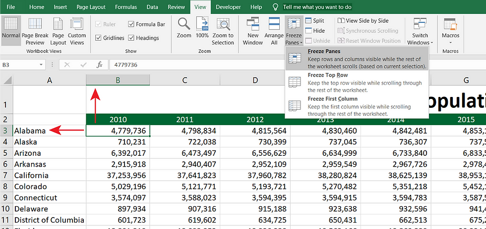
On the View Ribbon, click Freeze Panes, then select “Freeze Top Row” to freeze the top row. The top row will now stay at the top of the spreadsheet, no matter how much you scroll.

The same process can be done if you wanted the first column to stay in place. You would just click Freeze First Column.
When you want more than one column or one row, or when you want to have a combination of columns and rows, you select the Freeze Panes option. Excel will then freeze the row above the active cell and the column that’s to the left.

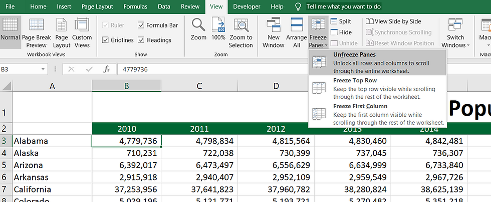
To remove the frozen panes, you can click Unfreeze Panes in the same section of Excel:

If you are into shortcuts, you can hit Alt, W, F, F for the freeze panes option, Alt, W, F, R to freeze the first row, and Alt, W, F, R for the first column. It might not seem like pressing that many buttons is quick, but you get used to it after a while and it becomes a much easier way to freeze panes fast.
Google Sheets
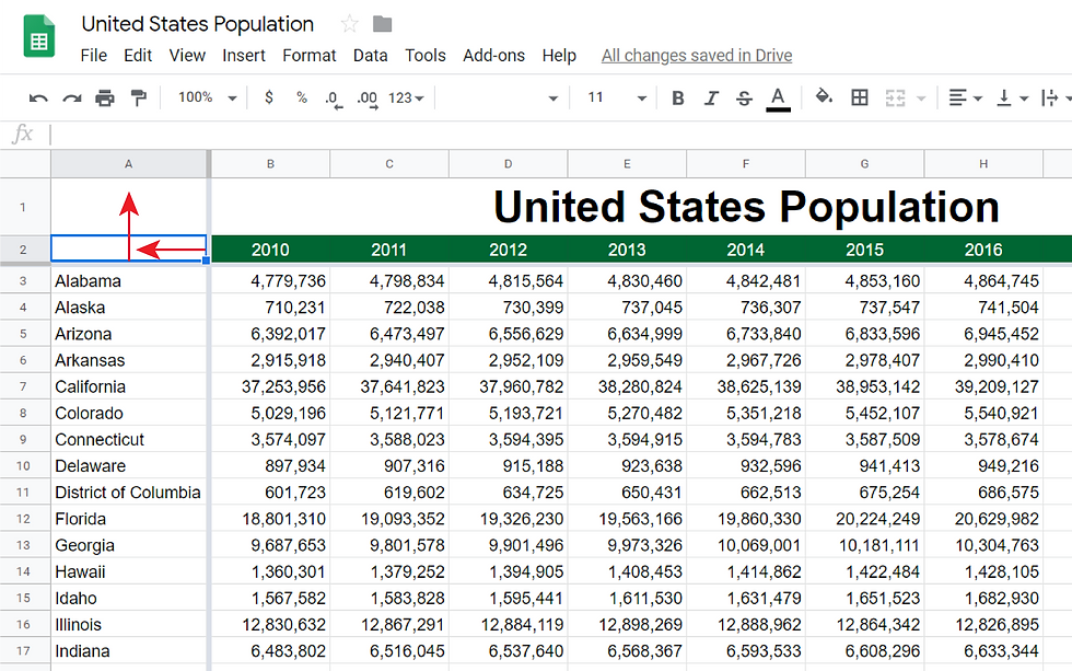
For those of you who use Google Sheets, the same concept exists, but is slightly different than Excel. To freeze panes, Click on the View Menu, and then select Freeze. Google Sheets gives you the option to select to freeze one or two rows or columns independently.

To unfreeze panes, you simply select “No Rows” or “No Columns” from the same menu.
Like Excel, you can customize the number of columns and rows that you freeze by selecting the “Up to current row”/“Up to current column” options. The difference with Excel is that when selecting the “Up to” option, Google Sheets will freeze the row below the active cell and will freeze the column to the right of the active cell.


Comments